DRP | Optimal Control

12 Jan 2026 in Projects

“Direct Reading Program in Mathematics at University of Florida”

Note: Use a desktop browser to view the interactive table of contents.

• How to mathematically optimize drug regimens using optimal control
• Reading Materials
  • Week 1
  • Week 2
  • Week 4
  • Week 5
  • Week 6
  • Week 7

Directed Reading Program (DRP) is mentoring initiative designed to give motivated undergraduates an opportunity to explore advanced mathematics topics under the guidance of a graduate stduent mentor.

Click this to learn more about DRP

How to mathematically optimize drug regimens using optimal control

🔬 Kyle Adams, Julia Bruner, Alexandra Haddad, Drew Nelson, A Hyeon Lauren Song, Kayla Adams

Institution: University of Florida

Semester: Spring 2026

Reading Materials

• DRP Reading.pdf
• NIH Permalink

Meetings: Every Tuesday Period 7(1:55-2:45) in LIT 368

Week 1

Reading

• “Introduction” Section of How to mathematically optimize drug regimens using optimal control, referred to as “main paper.”

• Guied Questions

  1. Why is optimal control preferred to standard “guess-and-check” methods?
  2. How “good” does a model have to be to apply optimal control to it?
  3. What does QSP stand for? Compare optimal control systems to QSP models.
  4. Take a look at the outline in figure 1. What questions or comments about it can you come up with?

---

Week 2

Date: January 20th, 2026

1. Optimal control theory: Optimal control theory is a powerful tool in mathematical optimization that allows us to find control functions that optimize the trajectory of a PDE with respect to some payoff function. There are multiple approaches this theory utilizes to find such a control, from the calculs of variations approach, to the Pontryagin Maximum principle and dynamic programming. Optimal Control Theory

2. Mechanistic (and semi-mechanistic) model: describe systems (biological in our case) based on known laws/concepts. Semi-mechanistic describe systems based on known laws, but are flexible to mechanisms that aren’t completely understood.

3. QSP Model: “Quantitative Systems Pharmacology” model: a mathematical model incorporates drug effects.
4. In silico (and in vitro, in vivo, etc): In sillico = “performed via computer simulation.” In vitro = “performed outside a living organism” (like a petri dish). In vivo = “performed within a living organism”

Here, we discussed comparing HIV Dosing Regimens constant therapy (traditional) and optimal therapy (optimizes treatment)

In HIV, constant therapy is continous drug pressure to suppress viral replication optimal control is time-varying, adaptive dosing that minimizes toxicity, resistance, and cost while maintaining control.

Objective Functionals: an objective functional allows researchers to summarize multiple goals such as maximizing healthy T cells whille minimizing infected cells and drug toxicity into one mathematical expresion to find the best possible treatment plan.

Applications in Disease Treatment:

• HIV Dosing: simulations show that optimal therapy can lead to better outcomes, such as maintaining higher T cells counts and lower infection levels, even when the total drug exposure (Area Under the Curve) remains the same as traditional methods.

• Chronic Myeloid Leukemia (CML): a comparison of various drug regimens demonstrates that a constrained optimal regimjen achieves a better value (a lower objective functional score) over five years compared to standard constant-dose regimens.

---

Week 4

Date: February 3rd, 2026

Artificial Pancreas: A real-world application of control theory (closed-loop insulin delivery) automatically adjust dosage based on real-time glucose monitoring. Algorithms for a Closed-Loop Artificial Pancreas: The Case for Model Predictive Control

Week 5

Date: Feburary 10th, 2026

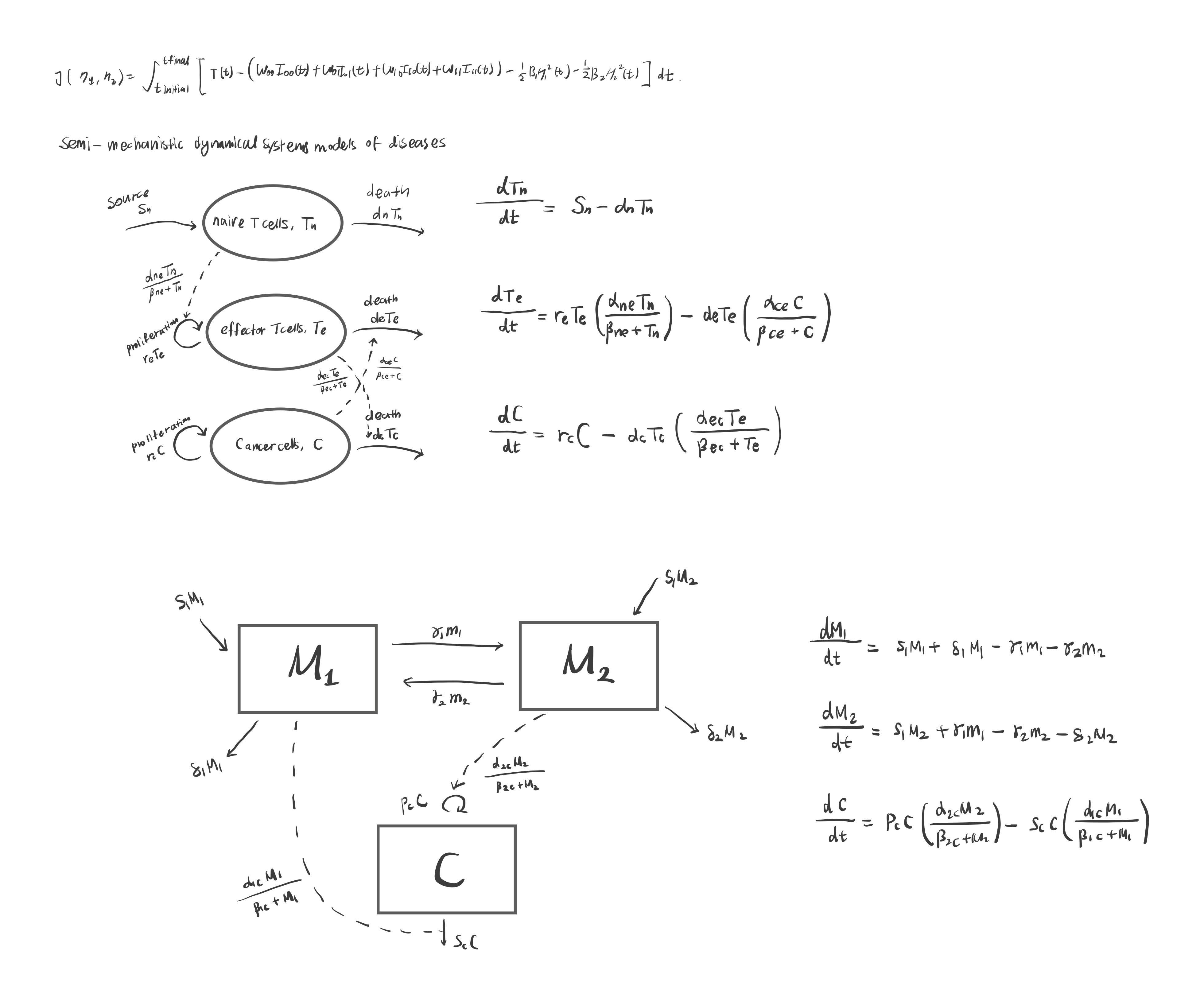
Practice drawing a model diagram, given the equations

Ways to model growth

Understanding Immune Dynamics in Liver Transplant Through Mahtematical Modeling

This is the model diagram, dynamics of graft rejection in liver transplantation.

Click link to read full article

Equation 5 models

Equation (5) models the rate of change of Tregs with respect to time. We assume a constant source rate of Tregs being recruited from outside of our model (pathway v). The factor z represents the natural loss of Tregs. The factor u, which is less than or equal to one, represents the lifespan-lengthening effect IL-2 has on tregs. We use a Michaelis-Menten term to ensure a bound on this effect size.

---

Week 6

Date: Feburary 17th, 2026

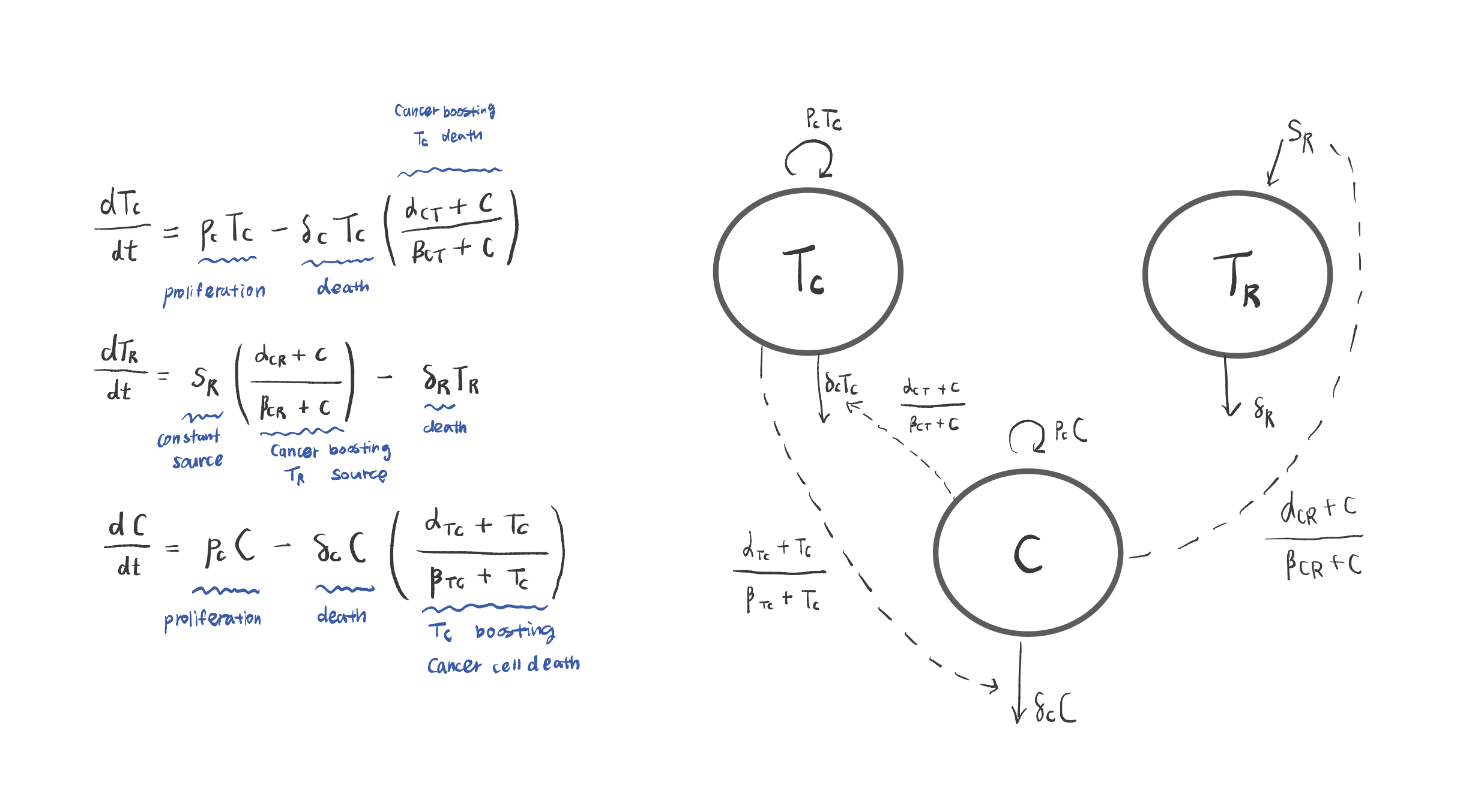
Reading the ODE for T_R (Regulatory T Cells)

$$\frac{dT_R}{dt} = \underbrace{s_R}_{v} - \underbrace{\delta_R T_R \left(1 - \frac{\alpha_{IR} I}{\beta_{IR} + I}\right)}_{z, \; u}$$

Breaking down each term:

• v — s_R: A constant source term. Regulatory T cells are produced at a baseline rate s_R, independent of other populations.
• z — δ_R T_R: Natural death/loss of T_R cells, proportional to current population size. δ_R is the death rate.
• u — (1 - α_IR·I / (β_IR + I)): A Michaelis-Menten style inhibition term. The cytokine I modulates the death rate — as I increases, this factor decreases, meaning I suppresses the loss of T_R cells.

Key question from the slides: What type of equation is this? What does its graph look like? The term αX / (β + X) is a saturating (hyperbolic) function — it rises steeply at first and levels off at a maximum value of α. This is the hallmark of Michaelis-Menten dynamics.

Reading the ODE for T_C (Cytotoxic T Cells)

$$\frac{dT_C}{dt} = \overbrace{\frac{\alpha_{HC} T_H}{\beta_{HC} + T_H}}^{k,l} + \overbrace{\gamma_C T_C \left(1 - \frac{T_C}{K_C}\right)}^{p} \left(\overbrace{-\frac{\alpha_{IC} I}{\beta_{IC} + I}}^{q}\right) - \overbrace{\delta_C T_C}^{t}$$

Breaking down each term:

• k, l — α_HC · T_H / (β_HC + T_H): Helper T cells (T_H) drive the activation/recruitment of cytotoxic T cells via Michaelis-Menten dynamics. The maximum activation rate is α_HC and the half-saturation threshold is β_HC.
• p — γ_C · T_C · (1 - T_C / K_C): Logistic proliferation of T_C cells. The population grows at rate γ_C but is self-limited by the carrying capacity K_C.
• q — (-α_IC · I / (β_IC + I)): Inhibition by cytokine I. This Michaelis-Menten term reduces proliferation — representing immune suppression.
• t — δ_C · T_C: Natural death of cytotoxic T cells at rate δ_C.

The Michaelis-Menten Function

A central building block for modeling saturating biological interactions is:

$$\frac{dY}{dt} = \frac{\alpha X}{\beta + X}$$

where α and β are constants, and X, Y are variables (e.g., cell populations or cytokine concentrations).

Exploring the parameters:

As X → ∞ (limit at infinity):

$$\lim_{X \to \infty} \frac{\alpha X}{\beta + X} = \alpha$$

The rate saturates at α — no matter how much X you add, the effect on Y cannot exceed α. This is why α is the maximum boosting effect X can have on Y.

When X = β (half-saturation point):

$$\frac{\alpha \cdot \beta}{\beta + \beta} = \frac{\alpha}{2}$$

At X = β, the rate is exactly half its maximum. This is why β is the threshold for half of the maximum boosting effect — it tells you how much X is needed to achieve 50% of the maximum response.

Michaelis-Menten Dynamics vs. Mass Action

These are two fundamentally different ways to model how one cell population affects another.

	Michaelis-Menten	Mass Action
Form	αX / (β + X)	c · X · Y
Behavior	Saturates at maximum α	Grows unboundedly with X and Y
Shape	Concave, asymptotic curve	Linear/superlinear growth
Biological interpretation	Receptor saturation; diminishing returns	Proportional to encounter rate between two populations
When to use	When there’s a biological maximum (e.g., receptor binding)	When interaction scales freely with both populations

Michaelis-Menten is appropriate when a biological process is rate-limited — for example, when receptors become saturated and adding more ligand produces diminishing returns. The curve starts steep and flattens toward α.

Mass Action assumes interactions are proportional to the product of two populations (c·XY). This can grow without bound and is more appropriate when physical encounter rates drive the interaction (e.g., predator-prey dynamics).

---

Week 7

Date: February 24th, 2026

Lagrange Multipliers are a technique for solving constrained optimization problems — that is, finding the maximum or minimum values of a function subject to some constraint. While the method has applications far beyond machine learning, it underpins several key derivations in the field.

Lagrange Multipliers with Computer Science (University of Toronto)

1. The Core Idea: Optimization With Rules

Normally, to find the peak of a hill (your objective function, E(x)), you simply look for the spot where the gradient is zero. But if you are told you must stay on a specific path (your constraint, g(x) = 0), the unconstrained peak might not lie on that path.

The key insight is to look for the point on the path where the hill’s slope and the path’s direction align in a very specific way.

1. The Trick: Parallel Gradients

Imagine the constraint is a circle drawn on a map. At any point on this circle, two gradients matter:

• ∇E (The Hill’s Slope): the direction of steepest ascent on the objective function.
• ∇g (The Path’s Direction): the direction perpendicular to your constraint curve.

At the optimal point on the path, these two gradients must be parallel. This means that any infinitesimal move you make that stays on the path won’t change your value on the objective function — you’ve found the best possible point.

Mathematically, this condition is expressed as:

$$\nabla E + \lambda \nabla g = 0$$

where λ (lambda) is an arbitrary scalar called the Lagrange Multiplier.

1. The Lagrangian

Instead of handling the objective and constraint separately, we combine them into a single function called the Lagrangian:

$$\mathcal{L}(x, \lambda) = E(x) + \lambda g(x)$$

By constructing this new function, we elegantly transform a constrained optimization problem into a standard unconstrained one — which is much easier to solve with standard calculus.

1. How to Solve It

To find the optimal point, we set the partial derivatives of L to zero:

• With respect to x → ensures the gradients of E and g are parallel (the core optimality condition).
• With respect to λ → enforces g(x) = 0, guaranteeing the solution actually lies on the constraint.

Solving this system of equations gives you the constrained optimum.

1. Worked Example: Minimizing on a Circle

Goal: Find the minimum of E(x, y) = x + y subject to the constraint g(x, y) = x² + y² - 1 = 0 (i.e., staying on the unit circle).

We form the Lagrangian:

$$\mathcal{L} = x + y + \lambda(x^2 + y^2 - 1)$$

Setting partial derivatives to zero and solving reveals that the optimum occurs where x = y, specifically at:

$$x = y = -\frac{1}{\sqrt{2}} \quad \text{(the minimum)}$$

E(x, y) = x + y — the objective function. Here we want to find its minimum value.

g(x, y) = x² + y² - 1 = 0 — the constraint, requiring all solutions to lie on the unit circle.

1. Why Does This Matter for Machine Learning?

Lagrange Multipliers appear throughout machine learning wherever optimization meets hard constraints. Two prominent examples:

• Principal Component Analysis (PCA): Finding the direction of maximum variance while constraining component vectors to unit length.
• Probability Distribution Estimation: Deriving distributions (e.g., maximum entropy models) where all probabilities must sum to exactly 1.

Understanding this technique provides a solid foundation for the mathematical machinery behind many ML algorithms.

Lagrange Multipliers with Biomathematics (ScienceDirect)